“Magnetic Loop Antenna”

Chapter 5: Automating Magnetic Loop Antenna (Part 2)

I introduced JR1OAO 2-port tuner system in the last chapter. I would like to go into a little more detail on how and why it works.

Tuner Operation Principle
The heart and soul of the system is Analog Devices AD8302 Gain and Phase Detector. This is a device to take two analog signals of up to 2.7GHz and compare their magnitude and phase, then outputs the error (difference) signals. This clever device has several usages including return loss / VSWR measurement, RF amplifier linearization, remote system monitoring, etc. but almost ideal for this tuner application. I will skip its internal details, but if you are interested, you can download the data sheet from http://www.analog.com/media/en/technical-documentation/data-sheets/AD8302.pdf .
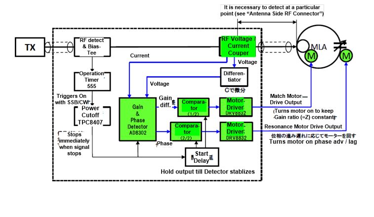
The tuner picks up the transmit RF signals voltage and current using its coupler module (current is picked up via toroidal core current transformer, and the voltage is picked up via a coupling capacitor). They are fed to the AD8302 to generate gain difference and phase difference voltages. Each are compared to preset voltage level and output via a pair of low power DC motor drivers. The driver outputs Pulse-Width-Modulation signals that drive a pair of DC motors (small, low power toy class motors) to manipulate the resonant capacitor and the coupling loop. The result will be reflected on the magnitude and phase difference sensed at the coupler module.  That forms the closed loop.

The circuit activates and functions whenever it detects RF power, as low as a few Watts, going through the coupler, then it controls two motors to achieve resonance and impedance match simultaneously, in a short time (in the order of 1 second). It is not necessary to explicitly transmit tuning carrier. Any transmission, any mode will trigger the action, including SSB, digital, FM and CW. So, wherever your moving your dial, the match will follow you automatically. That removes the biggest problem of the Mag Loop antenna, the narrow-banded-ness.

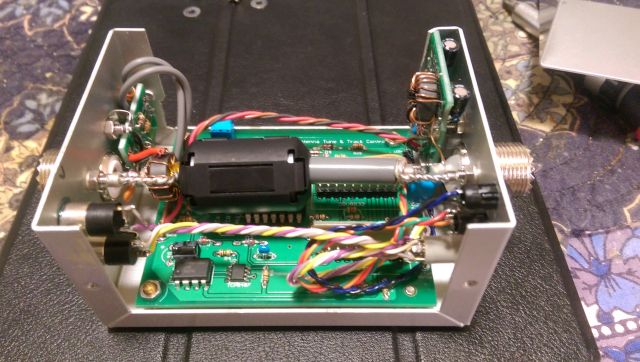
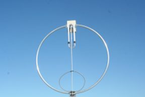
JR1OAO's "Super Tuner" for MLA

The system is purely analog, not using any processors. There are pros and cons associated with it, but one of the good things is it operates in extremely low power. And there is no stated power limit for the unit because it does not house any inductors or capacitors that take power loss. It also generates very little noise.

The unit is powered via coax feedline using a Bias-Tee. So, you do not have to pull a power cable to the unit. You just need to set up a supply side Bias-Tee by the transmitter. As stated, the unit runs on very low power so for a portable application, you may run with a battery, instead.

In order to further save power and another reason mentioned later, the unit is turned off when transmission power is not present. When the RF power is detected, it turns on after a short delay (waiting for the RF coupler to stabilize) to perform resonance / match operation.

Note there is no frequency measurement made anywhere in the system. So how does it know when the resonance is achieved?
Remember, in the last chapter when I discussed resonance? I said the resonance is the act of “removing reactance component from the complex impedance, Z = R”. When X is zero, Ohm’s law is valid and there is no phase difference between voltage and current. When AD8302 phase output is zero, the resonance is achieved. Clever, no?

More "Resonance and Match"
It is useful to bring about a visual aid to this concept of complex impedance and resonance / match. As much as I try to avoid digging too deep into technical pit, allow me to introduce Smith Chart.

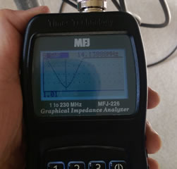
SWR Curve measured on MFJ-226
(reads SWR 1.01)

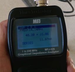
Measuring Complex Impedance
(reads 48 + j 1.06 ohm, almost a perfect match)

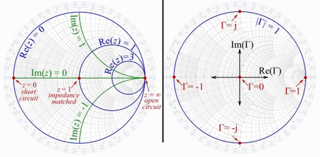
Smith Chart
When you express complex impedance as R + jX, you can plot this 2-dimensional entity in a X-Y coordinate with X-axis as R and Y-axis as X. Each access extends from negative to positive infinity and to see the whole picture, you will need an infinitely large sheet of paper. Not too convenient. Back in mid-20th century, Phillip Smith invented the chart where he plotted R and X axis in their entirety in a circle, called Gamma plane. It can display multiple parameters for various analyses.
While the use of paper Smith charts for solving the complex mathematics involved in matching problems, by now, has been largely replaced by software based methods, the Smith chart is still the preferred method of displaying how RF parameters behave at one or more frequencies, an alternative to tabulated numerical data.
In a typical “Z” Smith chart, R axis spans horizontally across the circle passing through its center. The right intersect with the circle represents infinite impedance, the left, 0 impedance. The center is where R = 1. It does not mean 1 ohm, but since the chart is “normalized”, for our applications, R = 1 means 50 ohm, or “impedance matched” point.
Just to be complete, there is a “Y” Smith chart, which plots admittance instead of impedance. It is a mirror image of “Z” chart,  but we’ll stick with Z chart for now.
The R axis, which I stated as center “line”, is actually a circle of infinite radius. There are (blue) circles touching the “infinite” impedance intersect with various diameters that represents specific R values. There are also (green) circle segments that cross the infinite impedance point at 90 degrees, that represent various values of X, or reactance. With that, we can plot any complex impedance R + jX as a point in the chart.

Smith Chart Basic (Ref: Wikipedia “Smith Chart”)

So now we can plot the complex impedance. What’s the big deal? It’s visual. You can grasp the story much faster than reading tabulated numbers. And convey more information than an SWR plot.
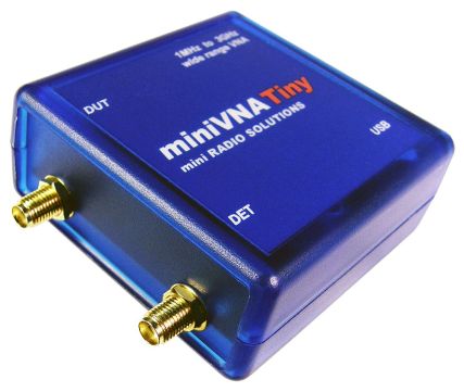
See the Smith Chart plots below. They are impedance of my MK-7 loop antenna across a range of frequency, obtained using my Mini VNA Tiny unit. This tiny blue box is a powerful dual-port VNA unit that can go up to 3GHz. Perhaps not a laboratory quality equipment, but powerful one for an amateur. I used that to plot the impedance of my loop antenna at various impedance matching configurations.

Mini VNA - Tiny
A small unit is a 2-port VNA that goes to 3GHz

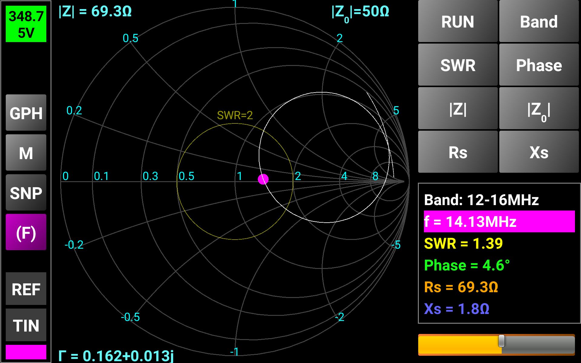
Smith Chart plot of optimally coupled loop antenna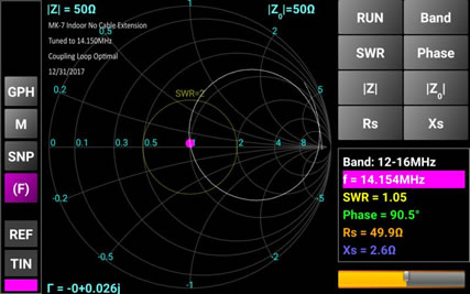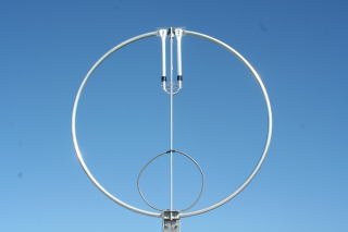

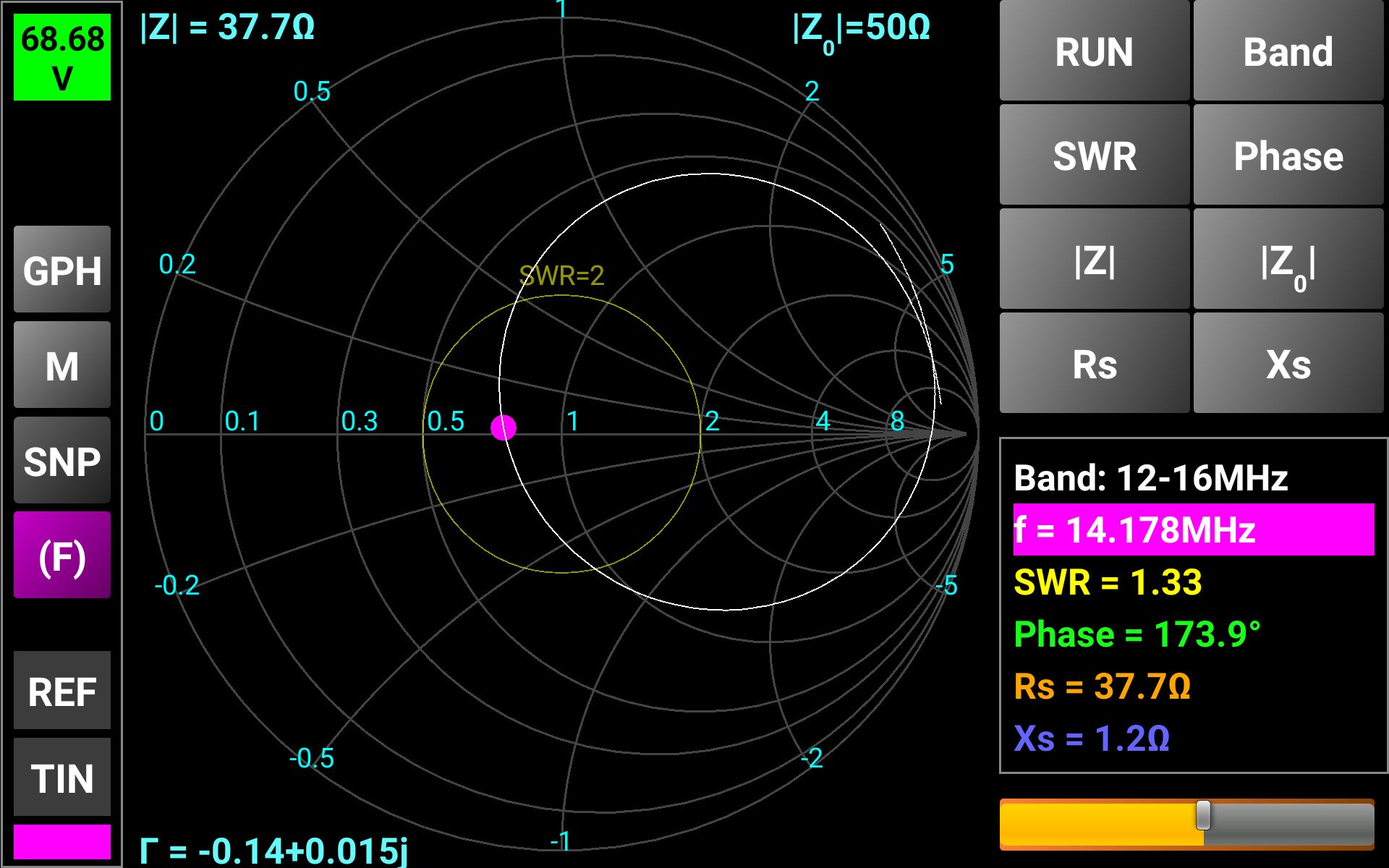
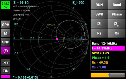
Smith Chart plot of loop antenna with loose coupling

Smith Chart plot of loop antenna with tight coupling

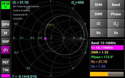Click on the Smith Charts on the left to see the full size plot. The white circle in the chart is the loop antenna impedance, as a function of frequency. The pink dot is roughly at the resonant frequency. Notice it intersects with R-axis at just about R=1.0 point. If you change the frequency, the impedance moves around the white circle. The antenna is in (IMHO) usable range for the frequency within yellow “SWR=2” circle. This circle is centered at R=1.0 (50 ohm) point and intersects with R-axis at R=0.5 (25 ohm) and R=2.0 (100 ohm). Anything inside this circle represents VSWR = 2.0 or less (good).

Back to the “Resonance & Match” discussion. The purpose of the tuning is to get this impedance circle to cross The R axis at R=1.0 at your desired operating frequency. The tuning action moves the “pink dot” around on the impedance circle.
Now, there is no guarantee that this impedance circle actually goes inside SWR=2 circle, or even intersects with R-axis at all. Without the matching, the loop antenna does not even look usable.

Do you remember, in the last chapter I talked about “changing the shape of coupling loop” to achieve the match? Let me show you…

The 3 charts on the left are the impedance plots for three different "shape" of the coupling loop. The tuning capacitor is tuned to about 14.15MHz for all 3 cases. Only the coupling loop shape is changed to display the difference.

Top one is "optimal", where the the top of impedance circle sits right around R=1.0.

One below is "loose coupling" case where the coupling loop is shaped skinny. Note the impedance circle diameter is shrunk and no longer passing through R=1.0 point.

The third one is "tight coupling" case where the coupling loop is shaped fat. Note the impedance circle gets bigger, and missed the R=1.0 point in the opposite direction.

For all 3 cases, the pink dot is placed at the lowest SWR point, and you see that the lower two cases cannot achieve 1.0 match.

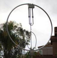
Coupling Loop Matching Strategies

So you see, the act of “impedance match” changes the diameter of the impedance circle. It should be adjusted so that the resonant point of the circle intersects with the R-axis at R=1.0. Then you have the perfect match.

Right now, without the tuner controlling the loop, I perform this resonance and impedance match manually. For the resonance part, the loop already has the trombone capacitor motorized, so I can use a remote to adjust. I can replace that with one of the motor driver outputs of the tuner. But for the impedance match, I need to motorize coupling loop. How do I do that?

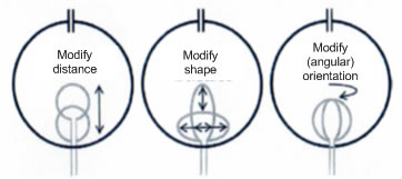
In the last chapter, I mentioned there are ways to vary the coupling to achieve desired impedance match. Three examples were mentioned:
- Modify distance between the main loop and the coupling loop
- Modify the shape of the coupling loop (my current scheme to do this manually)
- Modify the angular orientation between the main loop and the coupling loop

If you are operating in digital mode or CW, you may not have to be frequency agile, and for that, the narrow banded loop antenna, once the match is achieved, is very usable. For wider bandwidth modes like SSB, RTTY, SSTV, etc., would be a different story, so we want the auto tune capability for the antenna to be practical.

So there, you now caught up with my antenna project. I shall be updating as I make progress on the matching mechanism.
Meanwhile, there are lots of things to talk about small antennas, magentic loop or not.
So this writing continues...

Please, bring those comments, questions, suggestions to me: tak@w6si.com

To be Continued...